Fast trained neural network

Boris Zlotin; Ivan Nehrishnyi, Sr; Ivan Nehrishnyi, Jr & Vladimir Proseanic

Abstract

The paper is dedicated to the basic architecture of the artificial neural network of a new type – the Progressive Artificial Neural Network (PANN) – and its new training algorithm. The PANN architecture and its algorithm when applied together provide a significantly higher training speed than the known types of artificial neural networks and methods of their training. The results of testing the proposed network and its comparison with existing networks are given. For those who are interested in independent testing, information is provided allowing to download one of the variants of the proposed network.

1. Theoretical basis of fast neural network training

The artificial neural network (ANN) was mathematically confirmed as a universal approximating device in 1969 in [1]. At the same time, one of the major ANN limitations was revealed. As is known, each synapse in ANN has one synaptic weight. ANN training is performed by calculating and correcting these weights for the training image.For each next training image the same weights must be again corrected. Therefore, training is conducted through a large number of iterations. With training volume increase training time can grow exponentially.

In [2] and [3], a new neural network design is proposed, which differs from existing ANN by the fact there is a plurality of corrective weights at each synapse, and the corrective weights are selected by a special device (distributor) depending on the value of the input signal.

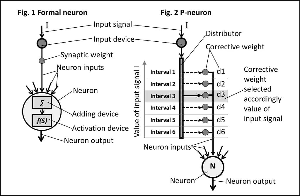
Figure 1 shows a well-known artificial formal neuron, which includes a summing device and an activation device, and Figure 2 shows a new artificial neuron, called p-neuron, proposed in [2] and [3].

In p-neuron, the signal from the input device is sent to the distributor, which estimates the value of the signal, refers it to one of the value intervals, and appropriately assigns a corrective weight corresponding to this signal. Figure 2 shows that a signal with a value corresponding to the value interval 3 selects the correcting weight d3.

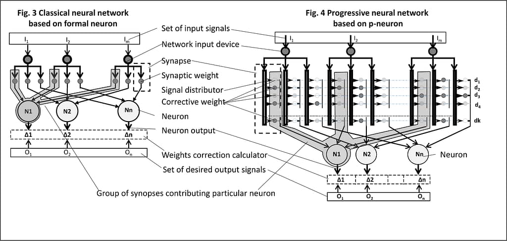
A new neural network has a classical neural architecture with p-neurons used in place of formal neurons. Figure 3 shows ANN with classical formal neurons, and Fig. 4 – a p-network with proposed p-neurons.

2. Training of the p-network

The P-network training, which that is shown in Fig. 4 differs significantly from the training of a classic ANN. Due to the presence of a plurality of corrective weights at each synapse, different input signals activate different weights. Input signals of the same value activate the same weights.

P-network training includes the following steps:

1. Input signals are sent to the distributors. Distributors activate weights at the synapses, depending on the value of the input signals. With other input signals, other weights at the synapses are activated. Values of these weights are sent to the neurons to which the synapses are connected.
   
2. Neurons form their output signals as a sum of corrective weights received by a given neuron
   
   ∑_n = ∑_{𝑖,𝑑,𝑛} 𝑊_{𝑖,𝑑,𝑛}
   
   Where:
   ∑_n – Neuron input signal;
   i – Corrective weight input index, which determines the signal input;
   d – Corrective weight interval index, which determines the value interval for the given signal;
   n – Corrective weight neuron index, which determines the neuron that received the signal;
   W_i,d,n – Corrective weight value;
   
3. Comparison of the received neuron output signals with the predefined desirable output signals and generation of correction signals for the group correction of corrective weights.
   
   Where, the group correction is a modification of the activated corrective weights associated with a given neuron, with each weight changing to the same value or multiplying by the same coefficient.
   
   Below are two exemplary and non-limiting variants of the formation and use of the group correction signals:
   
   Variant #1 – Formation and application of correction signals based on the difference between desirable output signals and obtained output sums, as follows:
   
   Calculation of the equal correction value ∆_n for all corrective weights contributing into the neuron n according to the equation:
   
   ∆_n = (O_n-∑_n)/ S
   
   Where:
   O_n – Desirable output signal corresponding to the neuron output sum ∑_n;
   S – Number of synapses connected to the neuron n.
   
   Variant #2 – Formation and application of corrective signals based on a ratio of desirable output signals versus obtained output sums as follows:
   
   Calculation of the equal correction value ∆_n for all corrective weights contributing into the neuron n according to the equation:
   
   ∆_n= O_n/∑_n
   
4. Correction of all weights connected to the given neuron. According to the first variant, Δ_n is added to the current weight value. In the second variant, the current weight value is multiplied by Δ_n. This nullifies the training error for the current image for a given neuron. In other words, instead of the gradient descent used in classical neural networks, which requires a large number of iterations, p-network provides a radical correction of the weights in one step.
   
5. Repeat steps 2 through 5 for all images. This completes the first training epoch. The corrected weights obtained during the network training with the first images of the epoch can be corrected by its training with the next images, and thus, training with previous images during one epoch may deteriorate. If the desirable accuracy is not achieved after the first training epoch, several more epochs can be carried out.

The simple method for calculating weight corrections that does not require iterative processes, provides a very fast completion of the training epochs. And the one-step correction of all active weights for the entire amount of the training error drastically reduces the number of epochs necessary for training.

3. Software implementation of a fast training neural network

The described p-network has been implemented in the software form using the Object Oriented Language. Fig. 5 represents the software implementation of the p-network in the Unified Modeling Language (UML).

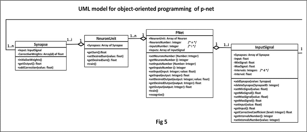
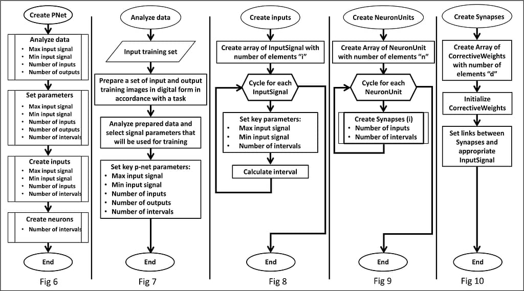
The UML model in Fig.5 shows the generated software objects, their relationships, as well as functions and parameters of these objects. In more detail, these steps are shown in Figures 6 –12, including:

• Fig. 6 – general sequence of p-network formation;
• Fig. 7 – analysis process, which allows to prepare data necessary for p-network formation;
• Fig. 8 – input signal processing, which makes it possible for the p-network to interact with the input data during its training and operation;
• Fig. 9 – formation of neuron units, including a neuron and a synapse with corrective weights, which provides p-network training and operation;
• Fig. 10 – creation of synapses with corrective weights.

Within the process the following classes of objects are formed:

• PNet;
• InputSignal;
• NeuronUnit;
• Synapse.

The formed class of objects NeuronUnit includes:

• Array of objects of the Synapse class;
• Neuron – a variable, in which adding is provided during training process;
• Calculator – a variable, in which the value of the expected sum is placed and where the calculations of the training corrections are being made.

The class NeuronUnit provides network training,including:

• Formation of neuron sums;
• Assignment of values of expected sums;
• Calculation of corrections;
• Introduction of corrections into corrective weights.

The formed class of objects Synapse includes:

• Array of corrective weights;
• Pointer directed to the synapse-related input.

The class Synapse provides the following functions:

• Initiation of corrective weights;
• Factors by weights multiplication;
• Weight correction.

The formed class of objects InputSignal includes:

• Array of pointers to the synapses connected with a given input;
• Variable where the value of input signal is placed;
• Values of potential minimum and maximum input signal;
• Number of intervals;
• Width of an interval.

The class InputSignal provides the following functions:

• Formation of the network structure, including:
  • Adding and removing links between an input and synapses;
  • Assignment of the number of intervals for the synapses of the given input.
• Assignment of values of parameters for the minimum and maximum input signal;
• Contribution into the network operation:
  • Setting the input signal;
  • Setting correction factors.

The formed class of objects PNet includes the array of object classes:

• NeuronUnit;
• InputSignal.

The class PNet provides the following functions:

• Specifies the number of objects in the class InputSignal;
• Specifies the number of objects in the class NeuronUnit;
• Provides group request of functions of the objects NeuronUnit and InputSignal.

In the training process, operation cycles are formed in which:

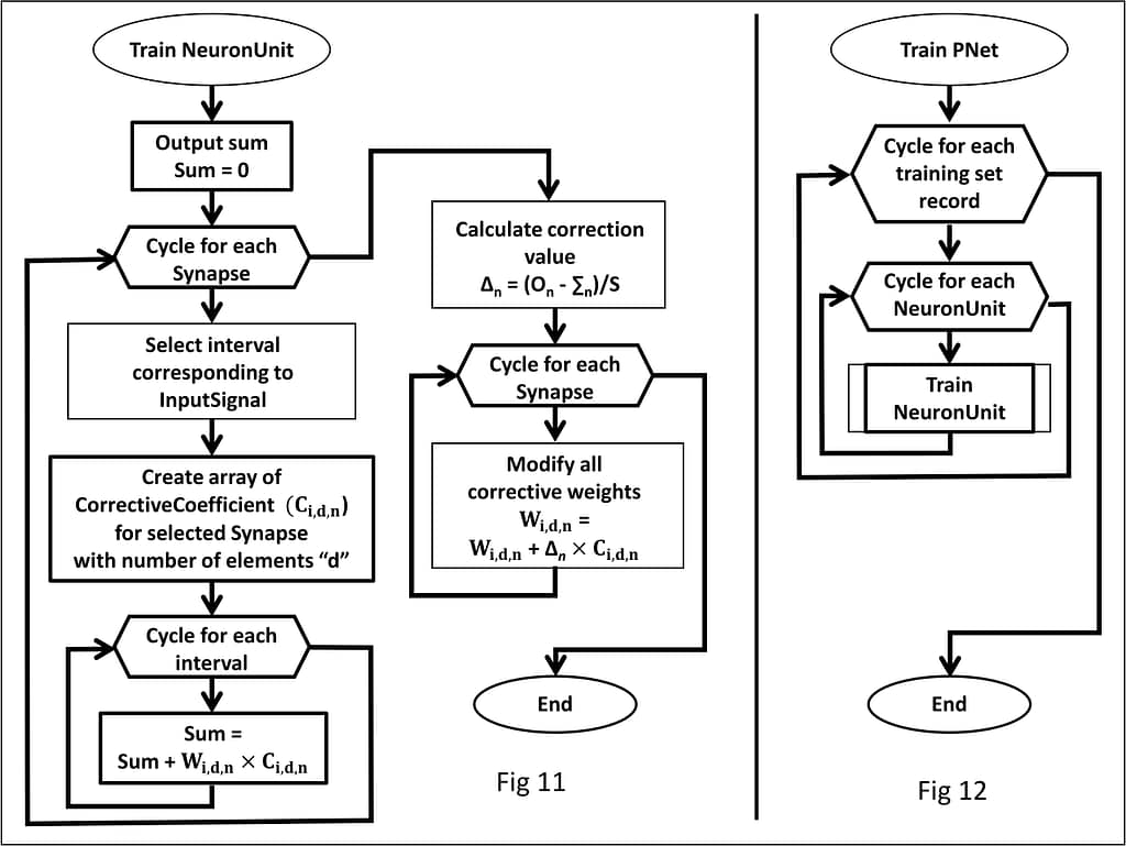
• The output of the neuron is formed, which is equal to zero prior to the start of the cycle. All the synapses contributing to the given NeuronUnit are reviewed, wherein for each synapse:
  • Distributor forms an array of correction factors based on the input signal.
  • All the weights coming to this synapse are reviewed, wherein for each weight the following operations are executed:
    • Multiplication of the weight value by the corresponding coefficient С_i,d,n;
    • The result of multiplication is added to the output sum of the neuron.
• Correction value ∆_n is calculated;
• The result of multiplication of the correction value ∆_n by the coefficient С_i,d,n is calculated (∆_n× С_i,d,n);
• All the synapses contributing to the given NeuronUnit are reviewed, wherein for each synapse:
  • All the weights coming to the synapse are reviewed, and each weight value is changed by the corresponding correction value.

Respectively:

• Fig. 11 – training process of a single neural unit in detail.
• Fig. 12 – general process of p-network training.

4. Test results

The experimental PANN built according to the above algorithm was implemented in Python.

The comparison was provided between Deep Learning ANN (DNN) based on advanced Google Tensor Flow technology and PANN. The results of comparison based on the standard statistical IRIS Test showed the following:

1. Training Error: PANN performance is comparable to the best results of the testedDNN;
2. Training Speed: PANN speed is at least 3,000 times higher than DNN.

The results of the tests are shown in the screenshot below.

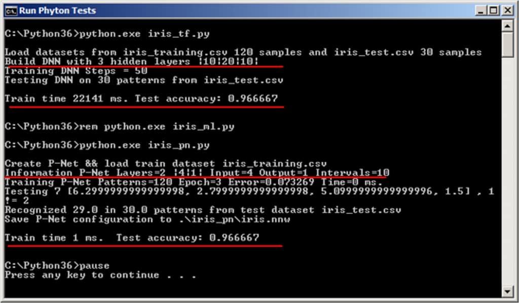
As can be seen, with the same accuracy, PANN training speed is 1 ms vs 22,141 ms for DNN.

The results are obtained on the computer with the following parameters:

• Windows 7 Home Premium
• Processor: Intel® Core™ i5 -337U CPU @ 1.80 GHz
• System type: 64-bit Operating System

It is apparent that on a different computer and with different processor download training time will be different.

Those who are interested in independent testing or in the non-commercial use of the new network can download one of its variants and user instructions here.

Discussion and conclusions

The tests have confirmed the theoretical expectations of a radical acceleration of network training by eliminating the need for iterative calculations. They also revealed additional benefits:

• Drastic decrease in the number of network training epochs necessary for the predefined accuracy of results. In some cases, the entire training was completed in 2-3 epochs, in some cases – in dozens of epochs. This provided additional reduction in training time.
• P-network has no need in activation function that is required in classical neural networks. Removing this function has further increased the training speed.
• PANN and the proposed training method can significantly accelerate the operation of various specialized neural networks, such as Hopfield and Kohonen networks, Boltzmann machine and adaptive networks. The network and its training method can be used in recognition, clustering and classification, prediction, associative information search, and the like, with additional partial network training in real time.

In addition, PANN application makes it possible to:

• Increase the computing power of computers, through the use of PANN-based computing blocks and cache memory systems.
• Save computing resources and reduce energy consumption.
• Create Large Databases with high performance, speed and reliability.

References

1. Marvin Minsky and Seymour Papert “Perceptrons: an introduction to computational geometry”, Cambridge, MA: MIT Press., 1969.
2. D. Pescianschi, A.Boudichevskaia, B. Zlotin, and V. Proseanic, “Analog and Digital Modeling of a Scalable Neural Network,” CSREA Press, US 2015.
3. Patent US9390373.
4. Patent US9619749.
5. Patent application US20170177998 A1.
6. International patent application PCT/US2015/19236, 06-Mar-2015.
7. International patent application PCT/US2017/36758, 09-JUN-2017.