Analog and Digital Modeling of a Scalable Neural Network

D. Pescianschi¹, A. Boudichevskaia^1,2, B. Zlotin¹, and V. Proseanic¹

¹ Progress Inc., West Bloomfield, MI, US
² Darmstadt University of Technology, Applied Plant Science, Darmstadt, Germany

Abstract

Proposed are the new types of fast training, scalable analog and digital artificial neural networks (p-networks) based on the new model of formal neuron, described in [1]. The p-network includes synapses with a plurality of weights, and devices of weight selection based on the intensity of the incoming signal. Versions of the p-networks are presented that are formed with resistance elements, such as, memristor elements. Also described are the matrix methods of training and operation for the proposed network. Training time for the new network is linearly dependent on the size of the network and the volume of data, in contrast to other models of artificial neural networks with the exponential dependence. Thus, p-network training time is dozens time faster than training time of the known networks. The obtained results can be applied in existing artificial neural networks, and in development of a neural microchip.

1. Structure of the p-network

The new model of the formal neuron (hereinafter – p-neuron), which is the core of the p-network is based on the following principles:

• Using multiple mediators in each synapse. In p-network the role of mediators may be carried by elements that are called corrective weights, which can be physically represented by electrical resistance, conductivity, voltage, electric charge, magnetic property, or other physical matter.
• Selection of corrective weight for each incoming signal at the synapse should be based on the value of the signal.
• The function of activation is not necessarily described by the sigmoid. Moreover, the output signal can be represented even by a simple sum of signals entering the neuron.
• Correction of the p-neuron weights – i.e., training is provided by not gradually correcting weight values for one image after another (gradual gradient descent), but with a one-step operation of error compensation during the retrograde signal. This takes into account only the information received by neuron in training from its synapses. However, the state of other neurons is not taken into account. Training the network to the next image does not depend on its training to the previous image. For each image used in training the complete compensation of training error is provided.
• Each neuron weight correction is provided by counter signals: the direct signal resulting from recognition by neuron of input image and the retrograde signal represented by the expected output. Correction of weights in analog form is provided as follows:
  • Direct signal obtained during recognition reduces the value of weights selected at the synapses in proportion to the magnitude of this signal.
  • Retrograde signal (the expected output signal) supplied to the output of a neuron increases the value of weights selected at the synapses in proportion to the magnitude of this retrograde signal.
• Independent correction of the weights of each neuron allows for complete parallelization of network training.

The above principles are the basis for the development of new training algorithms and allow creation of new p-network properties.

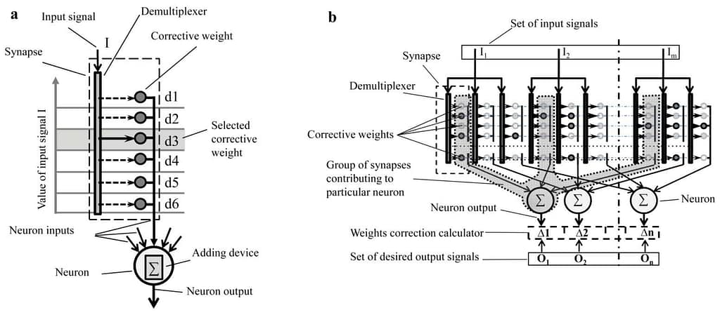
The Fig. 1a presents the proposed p-neuron. In the p-neuron the input signal reaches the device, which assesses the value of the signal and selects one of corrective weights corresponding to the value of this signal. The role of such a device can be performed, for example, by a demultiplexer. The Fig. 1a shows that the device selects the corrective weight 3 corresponding to the value of the input signal I. There can be a variant, wherein the selection of several corrective weights from available weights is provided.

By using the proposed p-neurons the network can be built with any desired topology, including topologies of classical neural networks that are built based of formal neurons. Fig. 1b a network including the proposed p-neurons – i.e., the p-network.

2. Analog modeling of the p-network

Biological network is completely analog by nature and its training and recognition mechanisms are accordingly analog. An example of artificial modeling of analog p-network could be the development of a p-network based on resistor elements, for example, memristors.

Each synapse stores information not in one weighting element (weight), but in a set of weights, each of which corresponds to a certain level (range of values) of the presynaptic signal. Resistors that are connected in parallel can be used as weight elements. The signals in this case would be coded by the currents in the circuits. Parallel connection of resistors provides the automated analog summation of signals in a neuron via summation of the currents on the conductor.

For each synapse it is necessary to provide two sets of weighting resistors: excitatory and inhibitory. Each such set of resistors is connected to the summing circuit of its own. Inhibitory signals are subtracted from the excitatory signals and result in the neuron output signal. Thus, to store not only positive but also negative resistance values, the circuit of the resistors should be bipolar. Otherwise active resistors would have been required to be capable of receiving negative values.

2.1. Recognition

The circuits of the upper three lines (Fig. 2a) have opposite sign to the circuits of the lower lines. Input signals X₁, X₂, X_m enter the control inputs of the device of choice, for example, the control inputs of the demultiplexers DMX₁, DMX₂, DMX_m, which select the circuits that become active (shown in bold). The power circuit A completes the selected circuits. The rest of the network circuits are disconnected. Thus, the set of parallel connected resistors are formed that are the selected weights of neurons. The currents are summed and form the outputs signals of neurons Y₁, Y₂, Y_n.

2.2. Training

The memristors can be used as weighting resistors. Correction of memristor resistors is provided via applying voltage pulses to the same circuits that are used for adding neuron signals. In other words, training of the memristor-based p-network can be provided in the same way as it happens in biological networks – by direct and retrograde signals. The network in Fig 2b is trained in two stages: recognition and training.

During recognition, memristors work as simple resistors (Fig. 2a). The input signals X₁, X₂, X_m are sent to control inputs of the demultiplexers DMX₁, DMX₂, DMX_m, which complete the circuits they have selected depending on the signal (indicated in bold). At the outputs the neurons’ current output signals Y₁, Y₂, Y_n are generated.

In the training mode network is trained in the same way as its biological prototype – by equilibrium process between the direct and retrograde signals. The immediate correction of weights is provided by voltage pulse U (y) that proportionally dependents on the signal y. As shown in Fig. 2b memristors in bipolar circuits have counter orientation. Thus, the training impulse increasing, for example, the resistance of the exciting circuit (reducing positive weights), at the same time reduces the resistance of inhibiting circuits (increases negative weights), and vice versa.

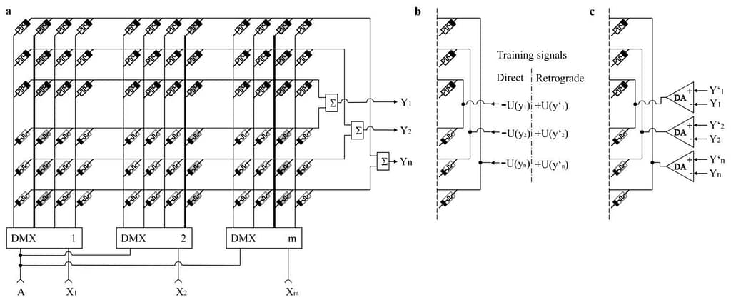
As in the biological prototype the direct training signal leads to weight reduction (synaptic depression), i.e. – to increased resistance in memristors of the excitatory circuit and to reduced resistance in memristors of the inhibiting circuit. For this purpose, the pulses – U (y_i) are applied to the neuron circuits, wherein, y_i is the output signal of the corresponding neuron.

Retrograde training signal, as in the biological prototype, leads to the weight increase (synaptic potentiation), i.e. – to reduced resistance in memristors of the excitatory circuit and to increased resistance in memristors of the inhibiting circuit. For this purpose, the neuron circuits are supplied with pulses + U (y^‘_i), wherein, y^‘_i – is the expected output signal of the corresponding neuron.

Correction of weights (memristors’ resistances), at training occurs only in complete circuits, i.e., in circuits already selected by demultiplexers DMX₁, DMX₂, DMX_m. This corresponds to the training of synapses only with selected mediators in natural networks.

2.3. Training optimization

The described mechanism (Fig. 2b) requires separation in time of the direct and the retrograde training signals. To combine these two steps (in order to increase the training speed), a differential amplifier (DA) can be used, one input of which is the current output signal of the neuron (Y_i), and the second input – the expected output signal of the neuron (Y^‘_i) (Fig. 2c).

This DA generates an output voltage proportional to the difference between the actual and the expected outputs, which is a measure of training error. In the training mode the pulse output voltage of the DA is sent to the memristor circuit, which leads to a change in memristor resistance. Moreover, the higher the error, the higher is the voltage, and therefore, the higher are the changes in memristor resistance. The voltage polarity of such pulse depends on the sign of the error.

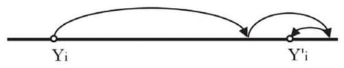
The error determines the voltage of correction pulse. Thus, the higher the neuron error, the higher is the voltage at the output of DA, the stronger are the changes at memristor circuit and, thus, the faster is the approach to precise training, i.e., absence of error. Training pulses are repeated until the predetermined threshold of training precision is not reached Fig. 3).

In addition to the conventional features of memristor chips, such as low power consumption and energy independence, memristor p-network has a number of new features:

• Analog recognition and training processes provide:
  • Significant increase in computing speed
  • The ability to store large volumes of data. It is well known that memristors allow storing resistance ranging from several ohms to several mega ohms, i.e., one memristor can store real numbers (several bytes of information).
• Increased yield of reliable microchips with p-network during their manufacture comparing to existing chips: Artificial neural network (ANN) does not use damaged connections during its training and can use memristors with deviated parameters without compromising the chip operation. Therefore, ANN is not very dependent on the imperfections of the manufacturing process.
• Durability of memristor neuro-chip: P-network ANN has substantially more weights on each synapse than the known ANNs. The information is distributed among a plurality of weights, and, therefore, loss or modification of the individual weights cause negligible distortion of information. Thus, some failures in memristor and connections in the process of application are compensated by other elements.
• Fast recover of memristor neuro-chip due to retraining of a defective microchip. Training speed of the proposed network enables training in real time.
• Resistance to the low accuracy of weight recording in individual memristors. P-network compensates such inaccuracy during training process due to the large number of elements, its architecture and training algorithm.
• Parallel memory operation: in contrast to the conventional method of memory operation, when the information can be read from individual nodes and written only to the exact node addresses, step by step, extracting and recording information in the memristor p-network is provided in parallel and without any node addresses. This allows processing in one step of the dozens’ times larger volumes of information than it is possible in the digital address memory. Thus, it also leads to increased speed.
• Conversion of memory from a device for storing information into a device for both: information storage, and processing. Moreover, unlike the sequence digital processing on the CPU and controllers, the process of parallel processing of information is implemented in the p-network. Thus, additional operations for the transfer of data between the CPU and memory are not required. Therefore, data processing is much faster.

3. Digital modelling of the p-network

It is easy to provide not only analog but also digital modeling of the p-network.

Moreover, its digital model can also process information in parallel.

The digital p-network for single and multi-processor systems can be described with the help of matrix algebra.

In particular, the array of memristor elements of Figure 2b can be represented as a two-dimensional matrix

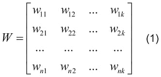
with dimensions of n x k, where n – the number of neurons (outputs), and k – the number of weights in a neuron. The signals in the circuits after de-multiplexers DMX₁, DMX₂, DMX_m can be represented as a binary matrix of one row I = [i₁ i₂ … i_k], with dimensions of 1 x k, i.e., as a line of ones and zeros, where the ones correspond to the selected complete circuits and zeros – to the rest of the (disconnected) circuits.

The vector of output signals can be represented by a matrix of one column

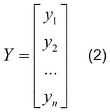
with dimensions of n x 1.

3.1. Recognition

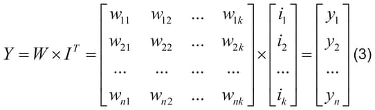
Recognition with the p-network is the summation of the matrix W elements for each row (neuron), and, only for active (selected) columns, which correspond to ones in the matrix I. Thus, the output image Y can result from multiplication of weight matrix W by the transposed matrix of input image I^T consisting of one column:

Batch recognition can be provided, that is, the recognition of a set of images at once. For this purpose, a number of input images can be presented as a matrix I with dimensions of v x k, where v – the number of recognizable images. Each row of the matrix I is a single image, subjected to recognition.

Thus,

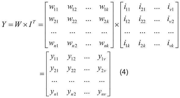
that is, multiplication of the matrix W, with dimensions of n xk, by the transposed matrix IT, with dimensions of k x v, produces the matrix Y, with dimensions of n x v, containing the required sums of selected elements in the rows of the weight matrix W for all recognizing images. Each column of the matrix Y is a single output image obtained by the recognition of the corresponding column of the matrix of the input images I.

3.2. Training

As described above, during training with the next image the retrograde signal completely compensates for the error, in the same way every time and uniformly (by the same impulse), thus, correcting all the selected weights of the neuron. In digital mode, the total error of the neuron is distributed between all selected weights of a neuron. That is, to obtain the correction value for each selected weight of the neuron it is necessary to calculate the total error for the neuron. Then, the resulting error is divided by the number of selected neuron weights to provide the correction value for the selected weights.

Error matrix E of the same dimensions as the matrix of the output image Y, is calculated, as follows:

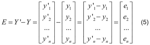
where Y’ – the matrix containing the image expected as the result of training, and Y – the matrix of the real output image. Matrixes E, Y’ and Y have the same dimensions.

Matrix of corrections (D), which contains the value of the necessary correction for each selected element of the matrix W, for each of the rows of the matrix (each neuron), is calculated by dividing each member of the matrix E by the m:

D = E / m, where m – the number of selected columns of the matrix W for the image (the number selected weights for a single output).

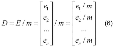
Where the error of each neuron is divided by the value of m.

To correct each selected element of the weight matrix W by the corrective value from the respective row of the matrix D, one should create the correction matrix C via multiplying the correction matrix D by the matrix of input image I.

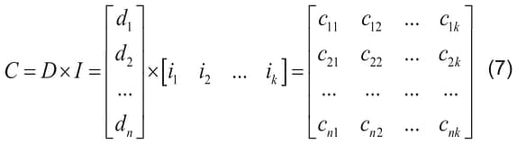
The matrix C has dimensions of n x k, as the weight matrix W; each element in each row of the matrix C is equal to 0, if it is in the unselected column, and is equal to an element of the matrix D of the corresponding row, when it is in the selected column. The selected column of the matrix W – is the column corresponding to the element of matrix I equal to one. The unselected column – is the column corresponding to the element of the matrix I equal to zero. Weight correction (training) is performed by adding the matrixes W and C, resulting in the matrix of corrected weights W’:

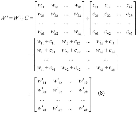
Thus, p-network is trained to one image in a single operation. The whole process of training a network to one image can be described by the formula:

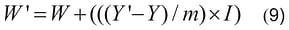
The same training operations are performed for all the images from the training set. The cycle including all the images is the training epoch. If the error level after one epoch is still too high, the training cycle for all the images is repeated.

Training and operation of multilayered networks have their own characteristics and need to be considered in a separate publication.

4. Test results

Experimental p-network, built on the given algorithm, has been developed as a single-threaded program. Testing was performed with laptop Dell Inspiron 5721, Intel CORE i5 1.80 GHz, Windows 7, by comparing the p-network with classical neural networks NeuroSolution and IBM SPSS Statistic 22. Tests were provided with the same data.

Training parameters were selected as follows: 1000 inputs, 20 outputs and 500 to 7000 images (records)

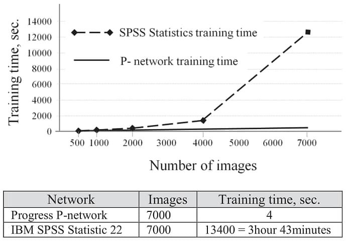
Test results are shown in the Figure 4. As seen in the Fig. 4, when the number of images is around 7000 the p-network is 3250 times faster. With increase in number of records the IBM SPSS Statistics 22 increases training time exponentially. The same increase in p-network increases training time linearly.

The tests have been conducted with the multithreaded versions of the p-network. In particular, the GPU version of the software was developed for running on video cards from NVIDIA supporting CUDA. With the GPU the 100% paralleling of the training and recognition processes was demonstrated. The linear speed increase has been demonstrated with the growth of the number of GPU. The increase is tens of times per GPU compared to the single-threaded version.

5. Conclusions

1. Proposed are the fast training scalable analog and digital models of a new type of artificial neural network (p-network), described in [1].
2. Presented are the analog and digital versions of networks formed with resistance elements, and in particular, with memristor elements.
3. The proposed networks include synapses with a plurality of weights, and devices of weight selection depending on the intensity of the incoming signal.
4. Presented are the matrix methods of training and operation for the proposed network.

This network provides:

• High speed training, due to multiple weights on each synapse and due to the new training algorithm.
• Training time is linearly dependent on the size of the network and the volume of data, in contrast to other models of ANN with the exponential dependence. The proposed network requires many times smaller number of training epochs than any classic ANN.
• Scalability, which allows building such networks of any size and complexity.
• Ease of implementation in the form of analog or digital circuits requiring no “external trainers” in the form of a computer, or a chip, which provide long-term and complex calculations.
• Batch processing of images, which significantly improves performance.

The proposed network is complementary to the memristors technology in creation of a highly reliable neural microchip. P-network also compensates for inaccuracies of manufacture and for unreliable operation of such microchips.

6. References

[1] D. Pescianschi, “Main principles of the general theory of neural network with internal feedback”, presented for the current congress.

Acknowledgements

We appreciate useful advice and support by S. Visnepolschi, A. Zusman, G. Peschanskiy. We are thankful for the support by the Progress Inc. working team and investors..